Particle MCMC for State Space Model Estimation

Building our first PMCMC algorithm!

This will be the final post of the series where everything will (hopefully) come together. In the first posts about HMMs and HSMMs, I explained the basics about said models. In the first blog post of my Inference in state space models series, I outlined a rough sketch on how to conduct parameter estimation for these models, and concluded that Bayesian methods are particularly suitable if we want to jointly sample the model parameter and the state sequence given the observed data. In the following post, I coded up a basic particle filter from scratch to sample the state sequence and, in my latest post, I implemented a framework to sample the corresponding model parameter. Please note that going forward you will need to import all Julia functions that we defined so far in order to make the code in this article work. If you do not want to copy paste code through all the articles, you can download the Julia scripts from my GitHub profile.

Explaining the estimation problem

Let us straight jump into the topic: the goal is to infer the posterior $P( s_{1:T}, \theta \mid e_{1:T})$. $\theta$ is, in our case, all the observation and transition parameter. If we assume univariate Normal observation distributions, we need to estimate $\mu$ and $\sigma$ for each state. In addition, we need to estimate the transition matrix, which I will keep fixed for now. You can also estimate this matrix if you extend our code in the MCMC part of the series for vector valued distributions. As a quick recap, we will use the particle filter from this post to sample the state trajectory, and the Metropolis sampler from this post to propose new model parameter. With the information gathered from both steps, we will either accept or reject this pair.

Coding the PMCMC framework

Let us start by loading all necessary libraries and defining two helper functions that we need in the PMCMC framework: a function to transfer the current values in our parameter container into the corresponding model distributions as well as a function to show all current values in this parameter container.

#Support function to transfer parameter into distributions
function get_distribution(μᵥ::Vector{ParamInfo}, σᵥ::Vector{ParamInfo})
    return [Normal(μᵥ[iter].value, σᵥ[iter].value) for iter in eachindex(μᵥ)]
end
get_distribution(param::HMMParameter) = get_distribution(param.μ, param.σ)

#Support function to grab all parameter in HMMParameter container
function get_parameter(parameter::HMMParameter)
    θ = Float64[]
    for field_name in fieldnames( typeof( parameter ) )
        sub_field = getfield(parameter, field_name )
        append!(θ, [sub_field[iter].value for iter in eachindex(sub_field) ] )
    end
    return θ
end

get_parameter (generic function with 1 method)

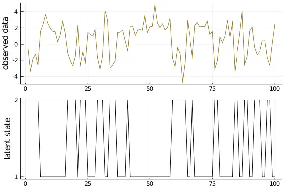
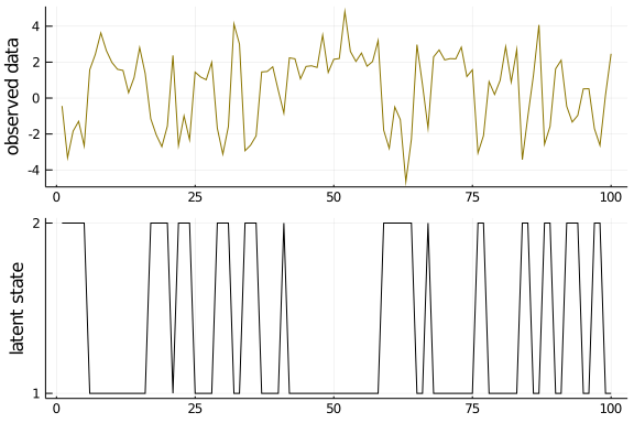
Neither of the two functions are needed to grasp the concept of PMCMC, but are useful for the sampling process. Next, let us sample the corresponding observed and latent data for some HMM. We will use these model parameter later on to compare the accuracy of our PMCMC algorithm:

#Generate data
T = 100
evidence_true =  [Normal(2., 1.), Normal(-2.,1.)]
transition_true = [ Categorical([0.85, 0.15]), Categorical([0.5, 0.5]) ]

s, e = sampleHMM(evidence_true, transition_true, T)

#Plot data
plot( layout=(2,1), label=false, margin=-2Plots.px)
plot!(e, ylabel="observed data", label=false, subplot=1, color="gold4")
plot!(s, yticks = (1:2), ylabel="latent state", label=false, subplot=2, color="black")

I explained this code already in an earlier post, so check this one out if there are any unclarities. I will now initialize the model parameter and the corresponding particle filter - note that there are many methods to do so, but for now we just initialize them manually, far enough away from the true parameter:

#Generate Initial parameter estimates - for univariate normal observations
μᵥ = [ParamInfo(3.0, Normal() ), ParamInfo(-3.0, Normal() )] #Initial value and Prior
σᵥ = [ParamInfo(1.5, Gamma(2,2) ), ParamInfo(2.0, Gamma(2,2) )] #Initial value and Prior
param_initial = HMMParameter(μᵥ, σᵥ)

#Generate initial state trajectory
evidence_current = get_distribution(param_initial)
transition_current = deepcopy(transition_true)
initial_current = Categorical( gth_solve( Matrix(get_transition_param(transition_current) ) ) )
pf = ParticleFilter(initial_current, transition_current, evidence_current)

You can check out this post if the code above is still unclear to you. Now all that is left to do is implementing the PMCMC sampling routine. I did my best to comment and make the code as clear as possible by adding comments at almost each line - the steps itself do not differ much from a standard Metropolis algorithm, so this function should be relatively straightforward to understand. The Unicode support for Julia also helps a lot here, as I could use a subscript t for variables that are defined in the transformed parameter space. Some more comments to understand the code a bit more clearly:

• The function input are the particle filter and the initial parameter guess we stated above. Additionally, the observed data will be used for the likelihood evaluation. Iterations stands for the number of samples that will be obtained. Scaling is a tuning parameter that states how big the proposal steps for the parameter will be. The larger the tuning parameter, the larger the movements. This influences the speed of convergence and acceptance rate into opposite directions. Check it out yourself by plugging in different values.

• The function output are the parameter and state trajectory samples. The results are pre-allocated at the beginning of the function in matrices called traces and will ultimately be used to check the accuracy of our algorithm.

• Before the loop starts, the initial parameter and state trajectory are assigned, and the log prior and likelihood given these values are calculated.

• The algorithm then proceeds by iteratively sampling new parameter and a state trajectory given the new parameter. Each iteration will be stored in the corresponding trace: if the step is accepted, the proposed parameter-trajectory pair is stored. Otherwise the current pair is stored.

• That’s it! Let us have a look:

function sampling(pf::ParticleFilter, parameter::HMMParameter,
                  observations::AbstractArray{T}; iterations = 5000, scaling = 1/4) where {T}
    ######################################## INITIALIZATION
    #initial trajectory and parameter container
    trace_trajectory =  zeros(Int64, size(observations, 1), iterations)
    trace_θ =  zeros(Float64, size( get_parameter(parameter), 1), iterations)
    #Initial initial prior, likelihood, parameter and trajectory
    logπₜ_current = calculate_logπₜ(parameter)
    θ_current = get_parameter(parameter)
    loglik_current, _, s_current = propose(pf, observations)
    #Initialize MCMC sampler
    θₜ_current = transform(parameter)
    mcmc = Metropolis(θₜ_current, scaling)

    ######################################## PROPAGATE THROUGH ITERATIONS
    for iter in Base.OneTo(iterations)

        #propose a trajectory given current parameter
        θₜ_proposed = propose(mcmc)
        #propose new parameter given current parameter - start by changing modelparameter in pf with current θₜ_proposed
        inverse_transform!(parameter, θₜ_proposed)
        pf.observations = get_distribution(parameter)
        logπₜ_proposed = calculate_logπₜ(parameter)
        loglik_proposed, _, s_proposed = propose(pf, observations)
        #Accept or reject proposed trajectory and parameter
        accept_ratio = min(1.0, exp( (loglik_proposed + logπₜ_proposed) - (loglik_current + logπₜ_current) ) )
        accept_maybe =  accept_ratio > rand()
        if accept_maybe
            θ_current = get_parameter(parameter)
            s_current = s_proposed
            logπₜ_current = logπₜ_proposed
            loglik_current = loglik_proposed
            #Set current θ_current as starting point for Metropolis algorithm
            mcmc.θₜ = θₜ_proposed #transform(parameter)
        end
        #Store trajectory and parameter in trace
        trace_trajectory[:, iter] = s_current
        trace_θ[:, iter] = θ_current
    end
    ########################################
    return trace_trajectory, trace_θ
end

sampling (generic function with 1 method)

Let us run this function with our initial parameter estimates:

trace_s, trace_θ = sampling(pf, param_initial, e; iterations = 3000, scaling = 1/4)

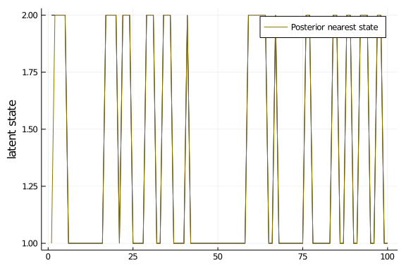
The final step is to check our posterior samples. I will do so by comparing the traces of the trajectories and the parameter against the parameter that have been used to generate the data:

#Check how well we did - trajectories
plot_latent = Plots.plot(layout=(1,1), legend=:topright)
Plots.plot!(s, ylabel="latent state", label=false, color="black")
Plots.plot!( round.( mean(trace_s; dims=2) ), color="gold4", label="Posterior nearest state")
plot_latent

#Check how well we did - θ
plot_θ = Plots.plot(layout=(2,1), legend=:topright)
Plots.hline!([2.,-2.], ylabel="μ", xlabel="", subplot=1, color="black", legend=false)
Plots.plot!( trace_θ[1:2,:]', color="gold4", label="Posterior draws", subplot=1, legend=false)

Plots.hline!([1.], ylabel="σ", xlabel="PMCMC Iterations", subplot=2, color="black", legend=false)
Plots.plot!( trace_θ[3:4,:]', color="gold4", label="Posterior draws", subplot=2, legend=false)
plot_θ

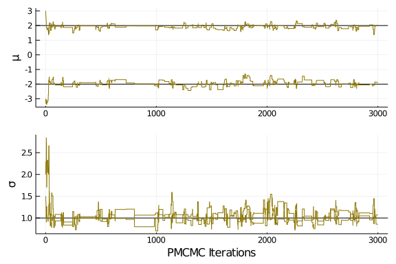
Not bad! Test it out yourself with different starting values, and check what happens if you change some of the tuning parameter, like the scaling size for the MCMC sampler, or the number of particles in the particle filter. In any case, you should now have a rough understanding about the PMCMC machinery, well done!

All done!

This concludes the mini series about inference on state space models. I hope this primer was enough to create some interest, shoot me a message if you have any comments! There are a lot of topics left to make further posts: we have not touched parameter initialization, expanding the algorithm to other state space models, or making the algorithm more efficient. So far, we have not even discussed forecasting! Though I have not decided on future blog posts yet, I will certainly expand on some of these topics. See you soon!