Bayesian Inference on State Space Models - Part 1
Bayesian Inference on State Space Models
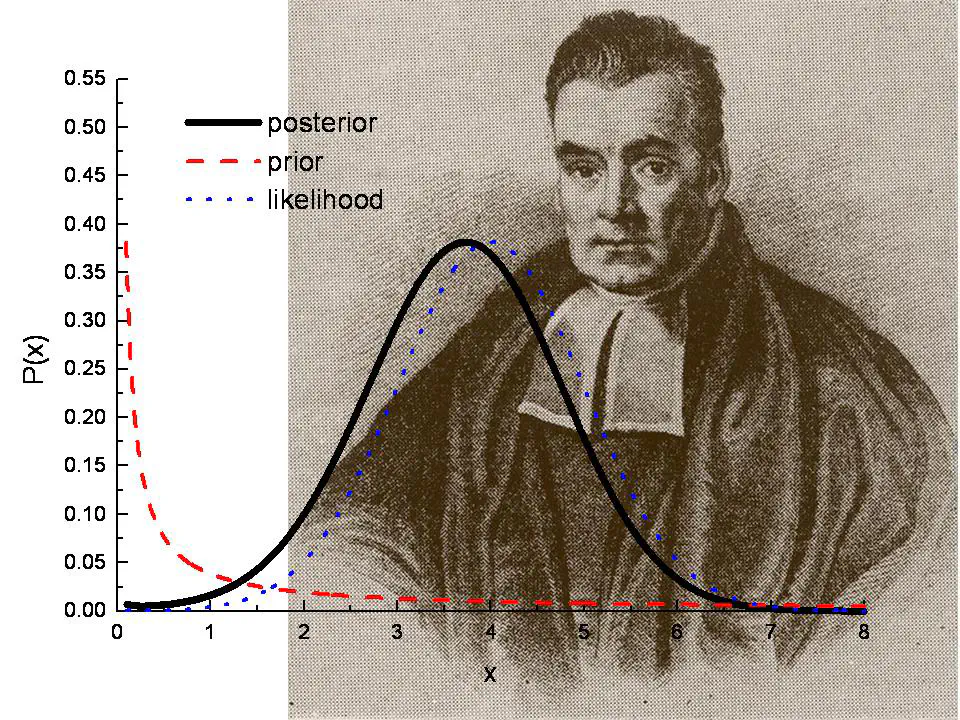 Image credit: statisticshowto
Hi there!
In my previous posts, I introduced two discrete state space model (SSM) variants: the hidden Markov model and hidden semi-Markov model. However, in all code examples, model parameter were already given - what happens if we need to estimate them? This post is the first of a series of four blog entries, in which I will explain a general framework to perform parameter inference on SSMs and implement a basic example for demonstration. Ideally, I would make all three posts as applied as my previous articles, but I have to use some theory in the beginning to make things easier going forward.
While SSMs are very flexible and can describe data with a complex structure, parameter estimation can be very challenging. Analytical forms of the corresponding likelihood functions are only available in special cases and, thus, standard parameter optimization routines might be unfeasible. Consequently, the major challenge in solving SSMs is the generally intractable likelihood function $p_{\theta}(e_{1:t}) = \int p_{\theta}(e_{1:t}, s_{1:t}) d s_{1:t}$, which integrates over the (unknown) latent state trajectory. As previously mentioned, $E_t$ is the observed data and $S_t$ the corresponding latent state.
So what can we do?
If both $E_t$ and $S_t$ follow a Normal distribution, one may analytically estimate the corresponding model parameter via the so called Kalman equations, but given these very specific assumptions, we will not concentrate on this special case going forward. If $S_{1:T}$ is discrete, then the most common point estimation technique is the EM-Algorithm. In this case, one can use common filtering techniques, explained in (Rabiner, 1989), to iteratively calculate state probabilities and update model parameter. Once the EM-Algorithm has reached some convergence criterion, one may estimate the most likely state trajectory given the estimated parameter. I will not go into much detail here because this procedure has been explained on many occasions and will instead refer to the literature above. However, both approaches do not work in many cases. The former technique only works with very specific model assumptions. The latter technique is not available in case $S_{1:T}$ is continuous. Moreover, even if the state sequence is discrete, summing out the state space might be computationally very challenging if the latent state structure is complex. In addition, one may not be able to write down the analytical forms of the updating equations for more complex state space models.
Another popular approach is to use Gibbs sampling, where one uses the previously mentioned filtering techniques to obtain a sample from the whole state trajectory $S_{1:T}$, and then sample model parameter conditional on this path. This technique suffers from the usually high autocorrelation within the model parameter vector and the state sequence. Moreover, ideally one would like to perform estimation jointly for the model parameter $\theta$ and the latent state space $S_{1:T}$, as both have a high interdependence as well. This is not feasible for either method that I mentioned so far. For a more in-depth discussion, an excellent comparison of point estimation and Bayesian techniques is given by (Ryden, 2008).
A general framework to perform inference on state space models
Given the statements above, I will now focus on a general approach to perform joint estimation on the model parameter and state trajectory of state space models, independent of the variate form of the latent space and the distributional assumptions on the observed variables. This is, to the best of my knowledge, only possible in a Bayesian setting, where we target the full joint posterior $P( s_{1:T}, \theta \mid e_{1:T})$ by iterating over the following steps:
-
- propose $\theta^{\star} \sim f(\theta^{\star} \mid \theta)$
-
- propose $S^\star_{1:T} \sim P(s^{\star}_{1:T} \mid \theta^{\star}, e_{1:T})$.
-
- and then accept this pair $(\theta^{\star}, s^{\star}_{1:T})$ with acceptance probability
$$ \begin{equation} \begin{split} A_{PMCMC} &= \frac{ P( s^{\star}_{1:T} \mid \theta^{\star}) }{ P(s_{1:T} \mid \theta ) } \frac{ P(e_{1:T} \mid s^{\star}_{1:T}, \theta^{\star}) }{ P(e_{1:T} \mid s_{1:T}, \theta ) } \frac{ P(s_{1:T} \mid e_{1:T}, \theta) }{ P(s^{\star}_{1:T} \mid e_{1:T}, \theta^{\star}) } \frac{P(\theta^{\star})}{P(\theta)} \frac{q(\theta \mid \theta^{\star})}{q(\theta^{\star} \mid \theta)} \\\\ &= \frac{P(e_{1:T} \mid \theta^{\star})}{P(e_{1:T} \mid \theta)} \frac{P(\theta^{\star})}{P(\theta)} \frac{q(\theta \mid \theta^{\star})}{q(\theta^{\star} \mid \theta)}. \\ \end{split} \end{equation} $$ Okay, but what does that even mean? In the first step, we propose a new parameter vector $\theta^{\star}$ from a MCMC proposal distribution. I will not go over the basics of MCMC, as this has been explained in many other articles, but we will implement an example in part 3 of this tutorial. Given this $\theta^{\star}$, we sample a new trajectory $s^\star_{1:T}$ and jointly accept this pair with the acceptance ratio from point 3. This framework allows to jointly sample $\theta$ and $S_{1:T}$, which was our goal in the first place. However, the in general intractable likelihood term is still contained in the acceptance probability in step 3, which is simplified by using the basic marginal likelihood identity (BMI) from (Chib, 1995). Consequently, the difficulty to obtain a sample from the posterior remains the same: we need to evaluate the (marginal) likelihood of the model.
The Particle MCMC idea
An alternative is to replace this (marginal) likelihood with an unbiased estimate $\hat{ \mathcal{L} }_\theta(e_{1:T}).$ In this setting, (Andrieu and Roberts, 2010) have shown the puzzling result that one can do so and still target the exact posterior distribution of interest, thereby opening a completely new research area now called ’exact approximate MCMC’. The algorithm that is used in this setting targets the full posterior and is known as Particle MCMC (PMCMC). Here, a particle filter (PF) is used to obtain a sample for $S_{1:T}$. A by-product of this procedure is that we also obtain an unbiased estimate for the likelihood. If you are more interested in PFs, have a look at the paper from (Doucet, A. and Johansen, 2011). For anyone wondering: as $p(s_{1:T} \mid e_{1:T}, \theta )$ is replaced with an approximation $\hat{p}(s_{1:T} \mid e_{1:T}, \theta )$, the approximation does not admit $p(s_{1:T}, \theta \mid e_{1:T})$ as invariant density, but this is corrected in the PMCMC algorithm via step 3.
Going forward
The PMCMC machinery provides a very powerful framework and cures many of the difficulties in the estimation paradigms mentioned at the beginning of this series. In reality, however, much of the performance depends on whether you find a good proposal distribution $ f( . \mid \theta)$ and $P(s^\star_{1:T} \mid \theta^{\star}, e_{1:T})$. Moreover, we have yet not mentioned how this machinery scales in the dimension of $\theta$ and $S_{1:T}$. These are all questions that I pursue in my own PhD studies, and we may venture through them once we know the very basics.
In the next blog post, we will implement a particle filter to do inference on the latent state trajectory. Going forward, we then talk about doing MCMC in this case, and implement a basic framework to sample from an unconstrained parameter space. Last but not least, we will combine all of this and apply a PMCMC algorithm on a standard HMM to obtain parameter estimates.
References
Andrieu, C. and Roberts, G. O. (2010). The pseudo-marginal approach for efficient monte carlo computations. Ann. Statist., 37(2):697-725.
Chib, S. (1995). Marginal likelihood from the gibbs output. Journal of the American Statistical Association, 90(432):1313-1321.
Doucet, A. and Johansen, A. (2011). A tutorial on particle filtering and smoothing: Fifteen years later.
Rabiner, L. R. (1989). A tutorial on hidden markov models and selected applications in speech recognition. Proceedings of the IEEE, 77(2):257-286.
Ryden, T. (2008). Em versus markov chain monte carlo for estimation of hidden markov models: A computational perspective. Bayesian Analysis, 3(4):659-688.
Patrick Aschermayr
Quantitative Researcher at Brevan Howard
Seeking a challenging and research-driven environment where I can develop and make a meaningful contribution.