Hi there!

In the last article, you got a first impression about state space models and, as an example, the basic hidden Markov model:

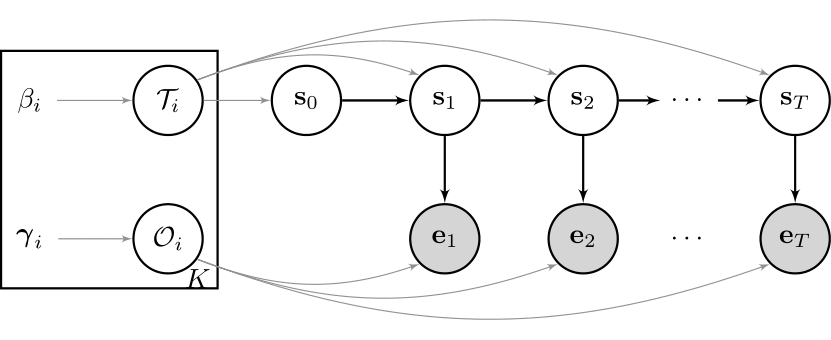
We already talked about various advantages of state space models, but - depending on the features of the underlying data that you want to model - basic HMMs just might not be good enough. Here is why:

A geometric duration distribution is a problem

Let us focus on the unobserved process, $S_t$, for now. We are interested in the actual time spent in a particular state. Let us calculate the probability that we are currently in state $i$ and remain here for the next two time steps. For a discrete 2-state, homogenous Markov chain, using the chain rule and the Markov assumption of the basic model, we can write: $$ \begin{equation} \begin{split} P( S_{t+3} = j, S_{t+2} = i, S_{t+1} = i \mid S_{t} = i ) &= P( S_{t+3} = j\mid S_{t+2} = i) P(S_{t+2} = i, \mid S_{t+1} = i) P( S_{t+1} = i \mid S_{t} = i ) \\ &= (1 - \tau_{ii}) * \tau_{ii}^2 \end{split} \label{eq:HMM_geom1} \end{equation} $$

In general, for $t+k$ steps: $$ \begin{equation} \begin{split} P( S_{t+k} = j, \dots, S_{t+1} = i \mid S_{t} = i ) &= (1 - \tau_{ii}) * \tau_{ii}^{k-1} \\ &= Geometric_{ \tau_{ii} }, \end{split} \label{eq:HMM_geom2} \end{equation} $$ where the geometric distribution has to be interpreted as the length of state duration up to and including the transition to the other state. Why is this a problem? The hidden states you model may switch more rapidly than you would like them to do. Even if you assign parameter very close to the boundaries of its support, the duration distribution will always implicitly be geometric. That makes it unsuitable if you want to model something that is supposed to stay in a particular state for a long time. As an example, let us say you want to model economic cycles of a developed country. You typically expect an expansion to last on average 5-10 years, but modelling such long durations is unfeasable with daily input data for an HMM. To circumvent this issue, one may use weekly or monthly data, but why give up data and essential information if alternatives are available?

From HMMs to HSMMs

As a solution, we can model these state duration probabilities explicitly. Such models are known as hidden semi-Markov models (HSMM), and they are a powerful generalization of the basic HMM. HSMMs have an additional latent variable, lets call it $D_t$ for duration that determines how long one may stay in any given state. $S_t$ will only have the Markov property while transitioning, otherwise it is determined by $D_t$. The tuple $\{ S_t, D_t \}$ forms a so-called semi-Markov chain. Let us visualize this:

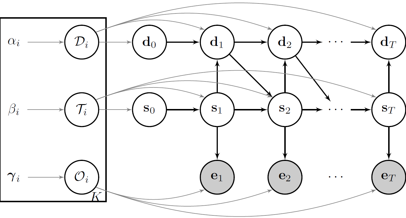
In an HSMM, transitions are allowed only at the end of each state, resulting in the following distributional forms:

where $\delta(a,b)$ is the Kronecker product and equals $1$ if $a = b$ and $0$ otherwise.

Note that, as we model the duration explicitly now, we have to slightly adjust the transition matrix that we used in the previous article. The diagonal elements of the transition matrix - the probability to remain in any given state in the next time step, which formally is depicted as $\tau_{i,i} = P(s_{t+1} = i \mid s_{t} = i)$ - are now set to 0. The rest of the row elements in the transition matrix still need to sum up to 1. If you have trouble understanding that, check out the code below.

Let us code!

To understand the code for sampling a single trajectory of said HSMM more clearly, keep reading:

• The function input are the model distributions stated above.

• The function output is a single trajectory of the observed and latent variables.

• Before we start the for-loop over time, we need to define the initial state. If the latent states of the data are conceived as a subsequence of a long-running process, the probability of the initial state should be set to the stationary state probabilities of this unobserved Markov chain. This plays an important part in the estimation paradigm, but for now we simply choose any of the available states with equal probability. Don’t worry if this sounds difficult - we will come back to it in a later article.

• The for-loop samples the new state given the old state, and then the observation given the new state, over time. The corresponding distributions are stated above.

• In the HSMM case, we check if the duration in the previous time step reached 0. If true, we sample a new state and duration given this state. If not, the current state continues, and we decrease the duration count by 1.

• That’s it! Let us have a look:

using Distributions

function sampleHSMM(evidence::Vector{<:Distribution}, duration::Vector{<:Distribution}, transition::Matrix{Float64}, T::Int64)
        #Initialize states and observations
        state = zeros(Int64, T)
        state_length = zeros(Int64, T)
        observation = zeros(Float64, T)

        #Sample initial s from initial distribution
        state[1] = rand( 1:size(transition, 1) ) #not further discussed here
        state_length[1] = rand( duration[ state[1] ] ) #not further discussed here
        observation[1] = rand( evidence[ state[1] ] )

        #Loop over Time Index
        for time in 2:T
                if state_length[time-1] > 0
                        state[time] = state[time-1]
                        state_length[time] = state_length[time-1] - 1
                        observation[time] = rand( evidence[ state[time] ] )
                else
                        state[time] = rand( Categorical( transition[ state[time-1], :] ) )
                        state_length[time] = rand( duration[ state[time] ] )
                        observation[time] = rand( evidence[ state[time] ] )
                end
        end
        #Return output
        return state, state_length, observation
end

sampleHSMM (generic function with 1 method)

Let us generate one sample path of said model. I am still using normal observation distributions, but added a third state so you can have a visual example from the transition matrix adjustment talk above. I will use a Negative Binomial distribution to model the state duration, but you are free to choose whatever you like best as long as the support lies on the non-negative Integers.

using Plots

T = 5000
evidence =  [Normal(0., .5), Normal(0.,1.), Normal(0.,2.)]
duration =  [NegativeBinomial(100., .2), NegativeBinomial(10., .05), NegativeBinomial(50.,0.5)]
transition = [0.0 0.5 0.5;
              0.8 0.0 0.2;
              0.8 0.2 0.0;]
state, state_length, observation = sampleHSMM(evidence, duration, transition, T)

plot( layout=(3,1), label=false, margin=-2Plots.px)
plot!(observation, ylabel="data", label=false, subplot=1, color="gold4")
plot!(state, yticks = (1:3), ylabel="state", label=false, subplot=2, color="black")
plot!(state_length, ylabel="duration", label=false, subplot=3, color="blue")

To see why the HSMM is a large improvement over the previous model, try to mimic the average state duration with the code that we used for the basic HMM model. Likewise, you can choose a geometric state duration in the example here to mimic the HMM case. While the latter is done easily, the former should almost be unfeasable. As always, you can download the full script from my GitHub account.

That’s it for today!

Well done! Initially, I wanted to write an article about several model extensions, but I quickly figured that this would be much too long for what I was planning to do, and therefore focused on HSMMs only in this post. I am going to gradually write follow-up posts on this one, as there exist many more state space models with an interesting structure, such as autoregressive or factorial HMMs. See you soon!