Welcome!

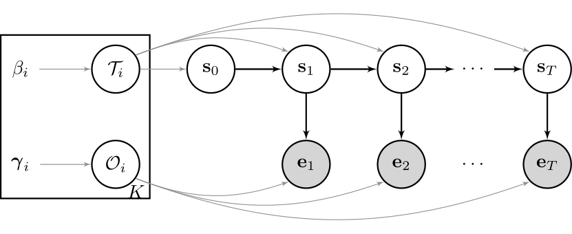
In my first series of posts, I will give a primer on state space models (SSM) that will lay a foundation in understanding upcoming posts about their variants, usefulness, methods to apply inference and forecasting possibilities. When talking about a state space model (SSM), people usually refer to a bivariate stochastic process $\{ E_t, S_t \}_{t = 1,2,\ldots ,T }$, where $S_t$ is an unobserved Markov chain and $E_t$ is an observed sequence of random variables. This may sounds difficult now, so let us look at a graphical example of one of the most well known SSMs out there - the so called Hidden Markov Model (HMM):

So, what are SSMs really?

Cool! To sum up the idea above in words, there is some unobserved process $S_t$ guiding the underlying data $E_t$. The Greek letters in the square box are the corresponding model parameter, which we assume to be fixed for now, and their priors. For example, maybe you own some shares of a company? Then the periodic changes in your portfolio, $e_t$, will be influenced by the current state of the economy, $s_t$. Hence, you may model this relationship as an HMM. There are many different variants of the model stated above, which I will discuss in future posts. One may include some autoregressive structure for the observation sequence, or one may decide to model the state sequence as a higher order Markov chain or even as a semi-Markov chain. Depending on the underlying data you want to model, one may also want to combine several of these ideas.

And why are they useful?

It turns out that having an underlying, unobserved process guiding some observed variables is a phenomenon that comes up naturally in many different areas. While I used an example from finance, there are many areas in genetics, anomaly detection and speech and pattern recognition, among others, where this structure comes up naturally and SSM can be applied successfully. Moreover, these models

• can handle structural breaks, shifts, or time-varying parameters of a model. Model parameter will adjust depending on the current state.

• allow you to model complex and nonlinear relationships.

• handle missing and irregular spaced data easily.

• can be used to do forecasting naturally due to their sequential setting.

• have interpretable structure to perform inference.

So even if someone is only interested in the observed sequence, the addition of a latent variable offers much additional flexibility that might not be feasable otherwise. This comes at the price that SSMs are, in general, computationally hard to estimate. I will go further into this topic in a separate post.

Sampling our very first State Space Model

For our first SMM, we will use observations that are normally distributed given the states. In this case, $S_t$ is a first order Markov chain, which can be depicted as a so called transition matrix $\tau$ . Each row in this matrix has a Categorical distribution, and the parameters thus have to sum up to 1 and are bounded between 0 and 1. $$ \begin{equation} \begin{split} & e_t \sim Normal(\mu_{s_t}, \sigma_{s_t} ) \\ & s_t \sim Categorical( \tau_{s_{t-1}}) \ \end{split} \end{equation} $$ Let’s write down a function that can generate sample paths of the HMM from above. I will mainly use Julia in my blog posts, as this programming language is incredibly fast and readable, and has some amazing features to make the life of anyone doing scientific computational research much easier. Here are some notes to help understand the code to sample a single trajectory of said HMM:

• The function input are the model distributions stated above.

• The function output is a single trajectory of the observed and latent variables.

• Before we start the for loop over time, we need to define the initial state. If the latent states of the data are conceived as a subsequence of a long-running process, the probability of the initial state should be set to the stationary state probabilities of this unobserved Markov chain. This plays an important part in the estimation paradigm, but for now we simply choose any of the available states with equal probability. Don’t worry if this sounds difficult for you - we will come back to it in a future post.

• The for loop samples the new state given the old state, and then the observation given the new state, over time. The corresponding distributions are stated above.

• That’s it! Let us have a look:

using Plots, Distributions

function sampleHMM(evidence::Vector{<:Distribution}, transition::Vector{<:Distribution}, T::Int64)
        #Initialize states and observations
        state = zeros(Int64, T)
        observation = zeros(Float64, T)

        #Sample initial s from initial distribution
        state[1] = rand( 1:length(transition) ) #not further discussed here
        observation[1] = rand( evidence[ state[1] ] )

        #Loop over Time Index
        for time in 2:T
                state[time] = rand( transition[ state[time-1] ] )
                observation[time] = rand( evidence[ state[time] ] )
        end
        return state, observation
end

sampleHMM (generic function with 1 method)

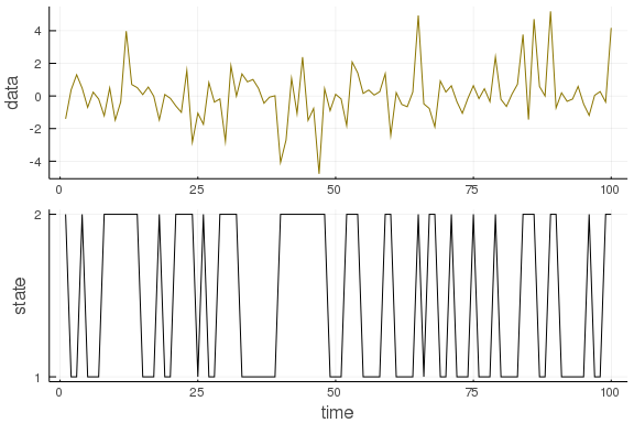
To round out this post, you can check out this function with different distributions and transition matrices:

T = 100
evidence =  [Normal(0., .5), Normal(0.,2.)]
transition = [ Categorical([0.7, 0.3]), Categorical([0.5, 0.5]) ]

state, observation = sampleHMM(evidence, transition, T)

plot( layout=(2,1), label=false, margin=-2Plots.px)
plot!(observation, ylabel="data", label=false, subplot=1, color="gold4")
plot!(state, yticks = (1:2), ylabel="state", xlabel="time", label=false, subplot=2, color="black")

You can download the full script from my GitHub account.

Going forward

We are off to a good start! Next time we will have a closer look at different variants of state space models and their subtle differences. This should give you a better understanding of possible use cases for SSMs!

In my first series of posts, I will give a primer on state space models (SSM) that will lay a foundation in understanding upcoming posts about their variants, usefulness, methods to apply inference and forecasting possibilities. When talking about a state space model (SSM), people usually refer to a bivariate stochastic process $\{ E_t, S_t \}_{t = 1,2,\ldots ,T }$, where $S_t$ is an unobserved Markov chain and $E_t$ is an observed sequence of random variables. This may sounds difficult now, so let us look at a graphical example of one of the most well known SSMs out there - the so called Hidden Markov Model (HMM):