Welcome back!

In my previous blog post, we explored a general framework to conduct parameter estimation on state space models (SSM). We call this framework Particle MCMC (PMCMC), and the three major steps to successfully apply this algorithm are as follows:

• 1. Find a good proposal distribution $f(\theta^{\star} \mid \theta)$ for $ \theta^{\star}$.
• 2. Find a good proposal distribution $P(s^\star_{1:T} \mid \theta^{\star}, e_{1:T})$ for $ S^{\star}_{1:T}$.
• 3. Find a sufficiently ‘good’ likelihood approximation $\hat{\mathcal{L}}$$_{\theta}(e_{1:T})$ that we can plug into the acceptance rate.

In this post, we will try to solve problems 2. and 3. simultaneously. Hence, we need to find a way to sample a state trajectory and get an approximation for the likelihood given the current parameter vector $\theta$. In order to use all the code we use here, please load all the functions from my introductory HMM article, or just include the corresponding HMM Julia file from my GitHub account.

Filtering the latent state trajectory

In PMCMC, a particle filter (PF) is used to first sample a trajectory $s^{\star}_{1:T}$ and then calculate an unbiased estimate of the corresponding likelihood. Note that unbiased does not mean our estimate is automatically ‘good’ enough, so there is quite a bit of ongoing research on how to keep the variance of particle filter likelihood estimates in check. For an in-depth explanation about PFs, I refer to (Doucet and Johansen, 2011), as explaining the whole machinery of it in detail is simply out of reach in a simple blog post.

In a nutshell, particle filters are usually used to solve filtering equations in the form of $$ \begin{equation} \begin{split} \pi_t( x_{1:t} ) &= \frac{ \tau_t(x_{1:t}) }{ Z_t }. \\ &= \frac{ w_{1:t} q_t(x_{1:t}) }{ Z_t }\ \end{split} \end{equation} $$

Here, the goal is to sequentially sample a sequence of random variables, $X_t, t \in (1,…, T)$ that come from a sequence of target probabilities $\pi_t( x_{1:t} )$ with the same computational complexity at each time step. The last part is crucial as we do not want to increase the computing time as more and more data comes in. You will notice I rewrote the equation by introducing $w_{1:t}=\frac{ \tau_t(x_{1:t}) }{ q_t(x_{1:t}) }$. Those familiar with importance sampling will likely understand why, but the reason we did so is because usually it is very difficult to sample from $\tau_t(x_{1:t})$. We introduce an easier distribution $q_t(x_{1:t})$ and reweight this distribution via $w_{1:t}$. Consequently, we need to find a good proposal distribution $q_t(x_{1:t})$, such that the computational complexity will not increase over time. A convenient by-product is that we can approximate the normalizing constant $Z_t$ with these weights: $$ \begin{equation} \hat{Z_t} = \frac{1}{t} \sum_{i=1}^{K} \frac{\tau_t(x_{1:t})}{q_t(x_{1:t})} = \frac{1}{t} \sum_{i=1}^{K} w_t(x^i_{1:t}). \end{equation} $$

In the basic HMM case, the joint distribution and the normalizing constant are of the form $\tau_t(x_{1:t}) = \prod_{k=1}^{t} f(s_k \mid s_{k-1}) g(e_k \mid s_k)$ and $Z = p(e_{1:t})$. Hence you can use the weights from above to approximate the likelihood that we need in the PMCMC sampler. In order to have a constant time complexity, one can use the Markovian properties of the latent states by imposing some transition density $q_{t}( x_{t} \mid x_{t-k})$ and propagating particles forward at each time step t. Afterwards, these particles will be weighted with the weight function we introduced above. Particles that are very unlikely given the observed data will then be replaced by more realistic particles - this has the effect that variance of our likelihood estimate will not be ’too’ large. After we propagated a bunch of particles forward up to the final time point T, we can sample one trajectory of these particles to get $P(s^{\star}_{1:T} \mid \theta^{\star}, e_{1:T})$ for our PMCMC algorithm.

If you read through the paper mentioned above, you will discover the optimal importance/proposal distribution in terms of minimising the variance of the likelihood estimate for processes with Markov property is $q(s_t \mid s_{t-1}, e_t) = p(s_t \mid s_{t-1}, e_t)$. This is usually not availabe, but gives some insight about good candidates. A common and simple choice is the so-called Bootstrap filter, which takes $q(s_t \mid s_{t-1}, e_t) = p(s_t \mid s_{t-1})$ and simplifies the corresponding particle weights to to $p(e_t \mid s_t)$. Both of these distributions are readily available in the HMM and HSMM case, so we jump straight into the coding section.

Coding our very first particle filter

The first thing that we need to define is the particle filter container itself. We will use the same style and structure as in our HMM post, and the advantage of the Bootstrap filter is that we can just plug in the model distributions from the HMM to define our PF. As a result, we define a field for the initial and transition distribution for our particles. The last field, observations, is used to weight the particles that we sample, so we can filter our particles that do not seem to capture the data well enough:

using Distributions, Parameters, Plots
import QuantEcon: gth_solve

mutable struct ParticleFilter
        initial         ::      Distributions.Distribution
        transition      ::      Vector{<:Distributions.Distribution}
        observations    ::      Vector{<:Distributions.Distribution}
end

In addition, we will define a helper function to calculate the corresponding weights in the log domain. This usually helps the numerical stability of the algorithm.

#Helper function
function logsumexp(arr::AbstractArray{T}) where {T <: Real}
max_arr = maximum(arr)
max_arr + log(sum(exp.(arr .- max_arr)))
end

function logmeanexp(arr::AbstractVector{T}) where {T <: Real}
    log( 1/size(arr, 1) ) + logsumexp( arr )
end

logsumexp (generic function with 1 method)

Good! Now we can straight jump into the actual code. As always, I do my best to make as many comments as possible, but to fully understand each step, there is probably no escape from reading the actual particle filter literature I mentioned above. Some comments to understand the code a bit more clearly:

• The function input are the particle filter we defined above, and some observed data that we use to weight the particles that we propagate forward.

• The function output is a log likelihood estimate, all the particle trajectories that we propagated forward, and a single trajectory that we will later on use in the PMCMC algorithm.

• Before we start the for loop, we pre-allocate the weights and the particles that we calculate later on. As you can see, we also normalize the weights, which I will denote with a subscript norm.

• The first particles are chosen from the initial distribution. If the latent states of the data are conceived as a subsequence of a long-running process, the probability of the initial state should be set to the stationary state probabilities of this unobserved Markov chain. Hence, this will be a function of the transition distribution of our model.

• The for-loop evolves around iteratively propagating particles forward and calculating the corresponding weights of the particles. As you can see, we will not always reweighting the particles at each iteration, but only if a certain threshold is achieved. This usually results in a even lower variance for our likelihood estimate. You can test this out yourself by altering the code and reweight at each iteration.

• That’s it! Let us have a look:

#Create a function to run a particle filter
function propose(pf::ParticleFilter, evidence::AbstractArray{T}; Nparticles=100, threshold=75) where {T<:Real}
        #Initialize variables
        @unpack initial, transition, observations = pf #Model parameter
        ℓlik = 0.0 #Log likelihood

        ℓweights = zeros(Float64, Nparticles)#Weights that are used to approximate log likelihood
        ℓweightsₙₒᵣₘ = similar(ℓweights)

        #initialize particles and sample first time point via initial distribution
        particles = zeros(Int64, size(evidence, 1), Nparticles )
        particles[1,:] =  rand(initial, Nparticles)

        #loop through time
        for t in 2:size(evidence, 1)

        #propagate particles forward
        particles[t, :] .= rand.( transition[ particles[t-1, :] ] )

        #Get new weights and calculate log likelihood
        ℓweights .= logpdf.( observations[ particles[t, :] ], evidence[t] )
        ℓweightsₙₒᵣₘ .= ℓweights .- logsumexp(ℓweights)
        ℓlik += logmeanexp(ℓweights) #add incremental likelihood

        #reweight particles if resampling threshold achieved
        if exp( -logsumexp(2. * ℓweightsₙₒᵣₘ) ) <= threshold
                paths = rand( Categorical( exp.(ℓweightsₙₒᵣₘ) ), Nparticles )
                particles .= particles[:, paths] #Whole trajectory!
        end

        end

        #Draw 1 trajectory path at the end
        path = rand( Categorical( exp.(ℓweightsₙₒᵣₘ) ) )
        trajectory = particles[:, path] #to keep type

        return ℓlik, particles, trajectory
end

propose (generic function with 1 method)

Perfect! With the weights, we can obtain the likelihood approximation, and with the particles, we can get the state trajectory that we need for the PMCMC algorithm. We still need to compute a function that translates our transition matrix to the initial distribution of the corresponding Markov chain. As such, we create a helper function so we can extract all the transition matrix parameter from our particle filter:

#Create a function so that we can obtain initial distribution from transition matrix
function get_transition_param(transitionᵥ::Vector{<:Categorical})
    return reduce(hcat, [transitionᵥ[iter].p for iter in eachindex(transitionᵥ)] )'
end

get_transition_param (generic function with 1 method)

Do not worry, this function is not necessary to understand the mechanics of PMCMC. It is just a convenient wrapper to create a transition matrix from all the parameter in our transition distribution. Now, let us check how good our algorithm works by first sampling some HMM data:

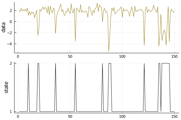
T = 150
HMMevidence =  [Normal(2., .5), Normal(-2.,2.)]
HMMtransition = [ Categorical([0.95, 0.05]), Categorical([0.5, 0.5]) ]

state, observation = sampleHMM(HMMevidence, HMMtransition, T)
plot( layout=(2,1), label=false, margin=-2Plots.px)
plot!(observation, ylabel="data", label=false, subplot=1, color="gold4")
plot!(state, yticks = (1:2), ylabel="state", label=false, subplot=2, color="black")

Next, let us create a Bootstrap particle filter with the corresponding transition and observation distribution from the HMM. If our code is correct, then the particle trajectories of our PF should be very close to the latent state sequence from the sample HMM data. As already mentioned, the initial distribution will be a function of the transition matrix:

#Initialize PF
pf = ParticleFilter( Categorical( gth_solve( Matrix(get_transition_param(HMMtransition) ) ) ),
                    HMMtransition,
                    HMMevidence
                    )

Cool! Now let us run the particle filter once and plot the propagated trajectories against the sample data:

ll, particles, trajectory = propose(pf, observation; Nparticles=500, threshold=500 )

Plots.plot(state, label="HMM latent states", xlabel="time", ylabel="latent state")
Plots.plot!( mean(particles; dims=2) , label="Particle Filter state trajectories")

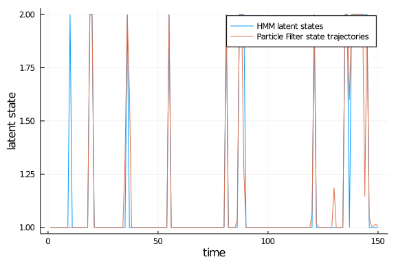
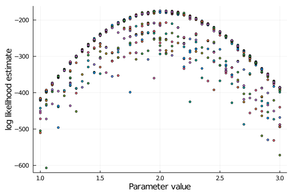
Good! The propagated particle trajectories from our algorithm are close to the sample data, exactly what we wanted to have. Play around with this yourself for different HMM parameter. There are, however, still a few aspects we have not yet dived into. For instance, how many particles do we need to achieve a “good” likelihood approximation? In the basic HMM case, we could actually calculate the likelihood exactly, and then check the solution against our approximation. This has been implemented many times, so it is easy to code this up yourself. I will instead focus on a different aspect: we said that our approximation is unbiased, but what about the variance of this estimate? There is a pretty good discussion and ideas on how to tune the number of particles on Professor Darren Wilkinson’s blog post about Particle MCMC. We already know that we can decrease the variance of our estimate by inflating the number of particles, but this comes at the cost of additional computing time - so how much is enough? Moreover, given we apply the particle filter in combination with a MCMC algorithm, it is important to know on whether the variance of our estimate is constant across the support of our parameter. To check this, we will initiate a grid of possible values for one parameter of your choice, and then run the particle filter several times for each element in the grid. In the end, we can visually check if the variance for these estimates is (a) low enough for your problem and (b) stays constant for a range of possible values:

#Check variance of likelihood estimate over a range of θ
function check_ll(pf::ParticleFilter, evidence::AbstractArray{T}, grid; runs = 20, Nparticles = 100) where {T<:Real}

        #Assign a matrix to store log likelihood estimate for each run
        ll_estimate = zeros(Float64, runs, length(grid))

        #Loop through the grid "runs" number of times, and assign the likelihood estimate to the preallocated matrix
        for iter in eachindex(grid)
                pf.observations[1] = Normal( grid[iter], pf.observations[1].σ)
                Base.Threads.@threads for idx in Base.OneTo(runs)
                        ll_estimate[idx, iter], _, _ = propose(pf, observation; Nparticles = Nparticles, threshold = Nparticles )
                end
        end

        #Return the log likelihood estimates
        return ll_estimate
end

grid = 1.0:0.05:3.0
ll_estimate = check_ll(pf, observation, grid; Nparticles = 500)
plot(grid, ll_estimate', seriestype = :scatter, ms=3.0, label="", xlabel="Parameter value", ylabel="log likelihood estimate")

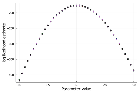
In this case, the variance does not seem to increase drastically given enough particles. You can see the contrast when assigning only a fraction of them:

ll_estimate = check_ll(pf, observation, grid; Nparticles = 50)
plot(grid, ll_estimate', seriestype = :scatter, ms=3.0, label="", xlabel="Parameter value", ylabel="log likelihood estimate")

In practice, you can choose the number of particles that you want to use by running a few trials for different parameter grids, but there are also methods to do so on the fly, some of them mentioned in my linked blog post above.

Nice one!

Wow, it took me a very long time to write this article, because it was extremely difficult to find a satisfying trade-off between making this post intuitive and explaining enough theory to ensure the code above makes any sense to you. To be honest, I would recommend reading one or two tutorials on particle filtering to fully understand the code, but I hope you could grasp the general goal through this blog post. That being said, the most difficult part is done! We can now sample a state trajectory and obtain a likelihood estimate for our MCMC algorithm for state space models. In part 3, we will use the most basic MCMC sampler and then finish the PMCMC algorithm to obtain estimates for a basic HMM. See you soon!

References

Doucet, A. and Johansen, A. (2011). A tutorial on particle filtering and smoothing: Fifteen years later.